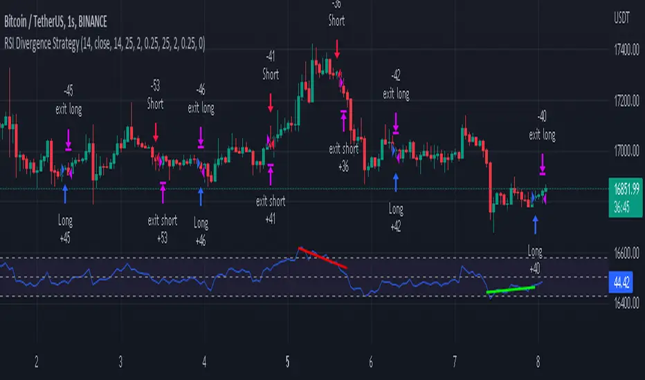
RSI Divergence Strategywhat is "RSI Divergence Strategy"?
it is a RSI strategy based this indicator:
what it does?
it gives buy or sell signals according to RSI Divergences. it also has different variables such as "take profit", "stop loss" and trailing stop loss.
how it does it?
it uses the "RSI Divergence" indicator to give signal. For detailed information on how it works, you can visit the link above. The quantity of the inputs is proportional to the rsi values. Long trades are directly traded with "RSI" value, while short poses are traded with "100-RSI" value.
How to use it?
The default settings are for scalp strategy but can be used for any type of trading strategy. you can develop different strategies by changing the sections. It is quite simple to use.
RSI length is length of RSİ
source is source of RSİ
RSİ Divergence lenght is length of line on the RSI
The "take profit", "stop" and "trailing stop" parts used in the "buy" group only affect buys. The "sell" group is similarly independent of the variables in the "buy" group.
The "zoom" section is used to enlarge or reduce the indicator. it only changes the appearance, it does not affect the results of the strategy.
在腳本中搜尋"the strat"
Fibonacci Zones EMA Zones StrategyThis idea is only for fun and learning purposes only.
The strategy represents 2 simple math formulas that are very simple. the "Fibo Formula" and the "EMA Formula" Please see source code for reference
I Feel like coders can learn a lot about developing strategies using this source code
This is to show that there is unlimited amount of variables and factors to a strategy and its all about working with probability.
Also to show that unlimited amount of conditions could be added to a strategy.
And unlimited amount of variables/factors with the settings that could change the results.
Rules are simple
Entry on close, Close/Entry must be in the blue Fibo Zone
Blue Fibonacci zone fully customizable
Other Conditions could be added involving EMA zones, Over Ema1, Under Ema1 etc..
TP/SL and Dates Fully Customizable
This script is just an idea fully for learning purposes.

Heikin Ashi SupertrendAbout this Strategy
This supertrend strategy uses the Heikin Ashi candles to generate the supertrend but enters and exits trades using normal candle close prices. If you use the standard built in Supertrend indicator on Heikin Ashi candles, it will produce very unrealistic backtesting results because it uses the Heikin Ashi prices instead of the real prices. However, by signaling the supertrend reversals using Heikin Ashi while using standard candle close prices for the entries and exits, it corrects the backtesting errors and gives you a more realistic equity curve. You should set the chart to use standard candles and then hide them (the strategy creates the candles).
This strategy includes:
Plotting of Heikin Ashi candles
Heikin Ashi Supertrend
Long and Short Entry Signals
Move stop loss after trade is X% in profit
Profit Target
Stop Loss
Built in Alertatron automation
Alertatron Trade Automation Integration
For Alertatron integration, be sure to configure the strategy settings and "Enable Webhook Messages" before creating an alert with {{strategy.order.alert_message}} in the body of your alert message. Be sure to enable webhooks and point it to your Incoming Alertatron webhook URL.
Notes
While this strategy does pretty well during trending markets, It's worth noting that the Buy and Hold ROI is much better during peak times of the bull market
Not financial advice. Do not risk more than you can afford to lose.

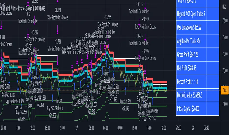
3Commas Bot DCA Backtester & Signals FREEThis is a DCA Strategy backtester + signals, built to emulate the 3Commas DCA bots. It uses your choice of 4 different buy signals, 2 of which can be adjusted in the settings. Everything is customizable so you can backtest specific settings with different buy signals and find the best performing strategy for your risk tolerance and capital. It can be used to backtest strategies on stocks as well, but just make sure your base order is larger than the share price for the entire backtesting range or it will not calculate properly.
You can use this template to code your own buy signals and then backtest them as a DCA strategy if you know some basic pine script.
The indicator shows all of your backtesting orders on the chart. The red line is your take profit level, the blue line is your average price level, the white line is your first order and the green lines are your average down orders. If you enable a stop loss in the settings your stop loss will be shown as an orange line once all of your average down orders have been hit, it will not be set until price has dipped below your covered trading range.
These levels update when things change during backtesting so you can visualize your strategy and how it would perform as well as see if your percentage deviation is large enough to cover dips. When backtesting trades are taken, the chart will show where they were taken(in backtesting) along with info on those trades such as the number each order is, the size of that order and the percentage deviation that order is from the initial buy.
SENDING SIGNALS TO 3COMMAS
Tradingview cannot sync this backtester to 3Commas and with the way alerts are setup for strategies on Tradingview, the best option for you to give signals to your bot would be to use this backtester to figure out what trigger you want to use and then setup that indicator separately to send alerts to your bot. All of the indicators used for signals in this backtester are available for free and can be configured to match this backtester and send alerts to 3Commas for you. Just make sure you set your alerts to once per bar close and don’t use less than a 15 second timeframe because then you could trigger the Tradingview threshold for alerts and get your alerts shut off.
You can also use this backtester with your own buy triggers if you know a little pine script. Just make copy of the script and code in your own buy signals and see how it backtests.
INFO PANEL FOR ANALYZING YOUR STRATEGY
The right hand side of the screen will show an info panel that shows a lot of different information so you can quickly see your bot settings and how it performed right on the screen.
In the top right corner you will see in purple your bot settings. These include your stoploss % if turned on, take profit %, average down order %, average down order % multiplier, volume multiplier, max number of orders allowed and size of your base order.
The top section of the first column “Current Trade” shows these stats: the open trade’s average price, the open trade’s take profit price, the open trade’s PNL, how far price is from your open tarde’s take profit level in percentage, your open position size and number of open orders.
The bottom section of the first column “Overall Performance” shows these stats: total number of trades taken during backtesting range, the largest amount of trades that were open at one time during backtesting, the max drawdown, the average number of bars per trade, gross profit, net profit, percent profit from your initial capital, current portfolio value and your initial capital.
CUSTOMIZABLE OPTIONS TO FIND THE PERFECT STRATEGY
Stoploss On/Off
This will turn your stoploss on or off. By default it is set to off and will not affect anything unless turned on.
Stoploss Percentage
This is the percentage below your final average down order price that will be set as a stoploss to keep your account from going too far in the red on big dips.
Take Profit Percentage - This is the percentage of profit you want the trade to hit before taking profit on your entire DCA trade. This level updates everytime you average down.
Average Down Percentage - This is the percentage that price has to drop from your initial order to initiate your first safety order. If the Average Down Percent Multiplier is set to 1 then this percentage will be the same for every average down order.
Average Down Percentage Multiplier - This multiplies your Average Down Percentage so each safety order needs a larger percentage deviation than the previous one. This keeps your buys closer together at the beginning and further apart when you hit more orders so you can extend your trading range but still be aggressive when price is going sideways.
Volume Multiplier Per New Order - This multiplies the size of each trade based on your base order. If you set it to a 2x multiplier then each average down order will be 2 times the size of the last one. So for example, a $100 base order with a 2x multiplier would have these values for the first 3 average down orders: 200, 400, 800.
Size Of Base Order - This is the size of your first position entry and will be used as a starting point for the volume multiplier. If your base order is $100 then it will buy $100 worth of whatever crypto you are backtesting this on. If you are looking at stock charts, you need to make sure your base order is higher than the share price across the entire backtesting range or it will not perform correctly.
Max Number Of Orders - This is the maximum number of orders the bot can take, including your base order. Adjust this to suit the amount of capital you are willing to allocate to your bot based on how much money it will require to run according to your bot settings.
TIPS ON HOW TO USE FOR BEST RESULTS
If you don’t have a lot of capital to work with, then use longer timeframes with a reasonable take profit percentage so that you don’t need a lot of average down orders. You can also try keeping the volume multiplier close to 1.
You can use the 3Commas dca bot settings page to see how much capital you will need for your strategy if you match it to the settings you have on this indicator. You can also check to see how much of a percentage deviation your bot is covering to make sure you have a reasonable range to trade in and orders to cover big dips. You can also check your coverage by seeing how far down the chart the green lines cover, which are your average down orders.
Make sure the initial capital in the properties tab of the settings has enough to cover all of your orders otherwise you will get unrealistic backtesting results. Also, make sure you leave the order size in the properties tab on contracts so it calculates your trades correctly. The only settings you need to touch in the properties tab is the initial capital. Unless you are trading somewhere that has lower commission fees, then you can change that to match, but leave all the other settings as is for it to function properly.
Increasing the volume multiplier will make your average price and take profit target follow the price action a lot closer as price falls, but it can also lead to having very large orders very quickly once you get into the 1.5-3x multiple range. Try using a high volume multiplier with less safety orders and you will get better results, however you need to have money on the sidelines to add on major dips to keep your bot turning a profit. Be very careful with this as greed and impatience will hurt your overall performance. This bot is meant to make money with lots of small wins so don’t get greedy and make sure you have enough money to cover large dips. If you are being aggressive with your bot, then I recommend only using 25% or less of your portfolio to trade aggressively and then use the smart trade feature on 3commas to add chunks of funds to your trades when price dips below your last safety order. Or if you want it to run without any supervision, then use lower volume multipliers and have lots of safety orders that can cover entire bear markets and still keep buying lower.
It’s a good idea to have some capital on the sidelines that you can add in when price dips quickly. This will help lower your average price and allow your bot to get out in profit quicker. 3Commas bot has a smart trade feature that will allow you to track your average price when adding extra funds and it will automatically update your other orders which is very convenient. Look at the longer timeframes when price dips and only add chunks at major areas where price is very likely to bounce. Or you can be aggressive when trading and add to your position when price dips and is at a likely bounce zone to maximize profits.
Only trade coins that have a good amount of liquidity as the larger your orders get, the harder it will be to sell if there isn’t much liquidity. Also, beware of how large your first order is as it will usually be a market order and can move the market if there is not much liquidity.
Since this bot takes a lot of trades and performs best when taking small profits consistently, you will need to factor in exchange fees. The bot is set to .5% commission(you can change this) on the buy and sell orders as most exchanges charge that amount. Some exchanges offer no fee trading on certain coins so be sure to look around for those so you can keep the commissions and maximize profits.
I strongly encourage you to try out a lot of different setting combinations across multiple different coins and do it across a few months to see how it would have performed under various market conditions. This will help you get a better idea of how much of a percentage deviation you’ll need to be able to cover to keep your bot running and making constant profits. You can also use the deep backtesting feature of the strategy panel to see how it would have done, but just beware that the info panel of the indicator will not reflect deep backtesting results, only the normal backtesting range.
MARKETS
This backtester can be used on any market including crypto, stocks, forex & futures. You just need to make sure your base order is larger than the share price when using this on things besides crypto.
TIMEFRAMES
This backtester can be used on all timeframes.
Channels Strategy [JoseMetal]============
ENGLISH
============
- Description:
This strategy is based on Bollinger Bands / Keltner Channel price "rebounds" (the idea of price bouncing from one band to another).
The strategy has several customizable options, which allows you to refine the strategy for your asset and timeframe.
You can customize settings for ALL indicators, Bollinger Bands (period and standard deviation), Keltner Channel (period and ATR multiplier) and ATR (period).
- AVAILABLE INDICATORS:
You can pick Bollinger Bands or Keltner Channels for the strategy, the chosen indicator will be plotted as well.
- CUSTOM CONDITIONS TO ENTER A POSITION:
1. Price breaks the band (low below lower band for LONG or high above higher band for SHORT).
2. Same as 1 but THEN (next candle) price closes INSIDE the bands.
3. Price breaks the band AND CLOSES OUT of the band (lower band for LONG and higher band for SHORT).
4. Same as 3 but THEN (next candle) price closes INSIDE the bands.
- STOP LOSS OPTIONS:
1. Previous wick (low of previous candle if LONG and high or previous candle if SHORT).
2. Extended band, you can customize settings for a second indicator with larger values to use it as STOP LOSS, for example, Bollinger Bands with 2 standard deviations to open positions and 3 for STOP LOSS.
3. ATR: you can pick average true ratio from a source (like closing price) with a multiplier to calculate STOP LOSS.
- TAKE PROFIT OPTIONS:
1. Opposite band (top band for LONGs, bottom band for SHORTs).
2. Moving average: Bollinger Bands simple moving average or Keltner Channel exponential moving average .
3. ATR: you can pick average true ratio from a source (like closing price) with a multiplier to calculate TAKE PROFIT.
- OTHER OPTIONS:
You can pick to trade only LONGs, only SHORTs, both or none (just indicator).
You can enable DYNAMIC TAKE PROFIT, which updates TAKE PROFIT on each candle, for example, if you pick "opposite band" as TAKE PROFIT, it'll update the TAKE PROFIT based on that, on every single new candle.
- Visual:
Bands shown will depend on the chosen indicator and it's settings.
ATR is only printed if used as STOP LOSS and/or TAKE PROFIT.
- Recommendations:
Recommended on DAILY timeframe , it works better with Keltner Channels rather than Bollinger Bands .
- Customization:
As you can see, almost everything is customizable, for colors and plotting styles check the "Style" tab.
Enjoy!
============
ESPAÑOL
============
- Descripción:
Esta estrategia se basa en los "rebotes" de precios en las Bandas de Bollinger / Canal de Keltner (la idea de que el precio rebote de una banda a otra).
La estrategia tiene varias opciones personalizables, lo que le permite refinar la estrategia para su activo y temporalidad favoritas.
Puedes personalizar la configuración de TODOS los indicadores, Bandas de Bollinger (periodo y desviación estándar), Canal de Keltner (periodo y multiplicador ATR) y ATR (periodo).
- INDICADORES DISPONIBLES:
Puedes elegir las Bandas de Bollinger o los Canales de Keltner para la estrategia, el indicador elegido será mostrado en pantalla.
- CONDICIONES PERSONALIZADAS PARA ENTRAR EN UNA POSICIÓN:
1. El precio rompe la banda (mínimo por debajo de la banda inferior para LONG o máximo por encima de la banda superior para SHORT).
2. Lo mismo que en el punto 1 pero ADEMÁS (en la siguiente vela) el precio cierra DENTRO de las bandas.
3. El precio rompe la banda Y CIERRA FUERA de la banda (banda inferior para LONG y banda superior para SHORT).
4. Igual que el 3 pero ADEMÁS (siguiente vela) el precio cierra DENTRO de las bandas.
- OPCIONES DE STOP LOSS:
1. Mecha anterior (mínimo de la vela anterior si es LONGy máximo de la vela anterior si es SHORT).
2. Banda extendida, puedes personalizar la configuración de un segundo indicador con valores más extensos para utilizarlo como STOP LOSS, por ejemplo, Bandas de Bollinger con 2 desviaciones estándar para abrir posiciones y 3 para STOP LOSS.
3. ATR: puedes elegir el average true ratio de una fuente (como el precio de cierre) con un multiplicador para calcular el STOP LOSS.
- OPCIONES DE TAKE PROFIT:
1. Banda opuesta (banda superior para LONGs, banda inferior para SHORTs).
2. Media móvil: media móvil simple de las Bandas de Bollinger o media móvil exponencial del Canal de Keltner .
3. ATR: se puede escoger el average true ratio de una fuente (como el precio de cierre) con un multiplicador para calcular el TAKE PROFIT.
- OTRAS OPCIONES:
Puedes elegir operar sólo con LONGs, sólo con SHORTs, ambos o ninguno (sólo el indicador).
Puedes activar el TAKE PROFIT DINÁMICO, que actualiza el TAKE PROFIT en cada vela, por ejemplo, si eliges "banda opuesta" como TAKE PROFIT, actualizará el TAKE PROFIT basado en eso, en cada nueva vela.
- Visual:
Las bandas mostradas dependerán del indicador elegido y de su configuración.
El ATR sólo se muestra si se utiliza como STOP LOSS y/o TAKE PROFIT.
- Recomendaciones:
Recomendada para temporalidad de DIARIO, funciona mejor con los Canales de Keltner que con las Bandas de Bollinger .
- Personalización:
Como puedes ver, casi todo es personalizable, para los colores y estilos de dibujo comprueba la pestaña "Estilo".
¡Que lo disfrutes!

[Sniper] SuperTrend + SSL Hybrid + QQE MODHi. I’m DuDu95.
**********************************************************************************
This is the script for the series called "Sniper".
*** What is "Sniper" Series? ***
"Sniper" series is the project that I’m going to start.
In "Sniper" Series, I’m going to "snipe and shoot" the youtuber’s strategy: to find out whether the youtuber’s video about strategy is "true or false".
Specifically, I’m going to do the things below.
1. Implement "Youtuber’s strategy" into pinescript code.
2. Then I will "backtest" and prove whether "the strategy really works" in the specific ticker (e.g. BTCUSDT) for the specific timeframe (e.g. 5m).
3. Based on the backtest result, I will rate and judge whether the youtube video is "true" or "false", and then rate the validity, reliability, robustness, of the strategy. (like a lie detector)
*** What is the purpose of this series? ***
1. To notify whether the strategy really works for the people who watched the youtube video.
2. To find and build my own scalping / day trading strategy that really works.
**********************************************************************************
*** Strategy Description ***
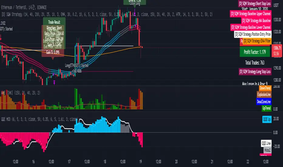
This strategy is from " QQE MOD + supertrend + ssl hybrid" by korean youtuber "코인투데이".
"코인투데이" claimed that this strategy will make you a lot of money in any crypto ticker in 15 minute timeframe.
### Entry Logic
1. Long Entry Logic
- Super Trend Short -> Long
- close > SSL Hybrid baseline upper k
- QQE MOD should be blue
2. Short Entry Logic
- Super Trend Long -> Short
- close < SSL Hybrid baseline lower k
- QQE MOD should be red
### Exit Logic
1. Long Exit Logic
- Super Trend Long -> Short
2. Short Entry Logic
- Super Trend Short -> Long
### StopLoss
1. Can Choose Stop Loss Type: Percent, ATR, Previous Low / High.
2. Can Chosse inputs of each Stop Loss Type.
### Take Profit
1. Can set Risk Reward Ratio for Take Profit.
- To simplify backtest, I erased all other options except RR Ratio.
- You can add Take Profit Logic by adding options in the code.
2. Can set Take Profit Quantity.
### Risk Manangement
1. Can choose whether to use Risk Manangement Logic.
- This controls the Quantity of the Entry.
- e.g. If you want to take 3% risk per trade and stop loss price is 6% below the long entry price,
then 50% of your equity will be used for trade.
2. Can choose How much risk you would take per trade.
### Plot
1. Added Labels to check the data of entry / exit positions.
2. Changed and Added color different from the original one. (green: #02732A, red: #D92332, yellow: #F2E313)
3. SuperTrend and SSL Hybrid Baseline is by default drawn on the chart.
4. If you check EMA filter, EMA would be drawn on the chart.
5. Should add QQE MOD indicator manually if you want to see QQE MOD.
**********************************************************************************
*** Rating: True or False?
### Rating:
→ 3.5 / 5 (0 = Trash, 1 = Bad, 2 = Not Good, 3 = Good, 4 = Great, 5 = Excellent)
### True or False?
→ True but not a 'perfect true'.
→ It did made a small profit on 15 minute timeframe. But it made a profit so it's true.
→ It worked well in longer timeframe. I think super trend works well so I will work on this further.
### Better Option?
→ Use this for Day trading or Swing Trading, not for Scalping. (Bigger Timeframe)
→ Although the result was not good at 15 minute timeframe, it was quite profitable in 1h, 2h, 4h, 8h, 1d timeframe.
→ Crypto like BTC, ETH was ok.
→ The result was better when I use EMA filter.
### Robust?
→ Yes. Although result was super bad in 5m timeframe, backtest result was "consistently" profitable on longer timeframe (when timeframe was bigger than 15m, it was profitable).
→ Also, MDD was good under risk management option on.
**********************************************************************************
*** Conclusion?
→ I recommend you not to use this on short timeframe as the youtuber first mentioned.
→ In my opinion, I can use on longer timeframe like 2h or bigger with EMA filter, stoploss and risk management.

[Sniper] SSL Hybrid + QQE MOD + Waddah Attar StrategyHi. I’m DuDu95.
**********************************************************************************
This is the script for the series called "Sniper".
*** What is "Sniper" Series? ***
"Sniper" series is the project that I’m going to start.
In "Sniper" Series, I’m going to "snipe and shoot" the youtuber’s strategy: to find out whether the youtuber’s video about strategy is "true or false".
Specifically, I’m going to do the things below.
1. Implement "Youtuber’s strategy" into pinescript code.
2. Then I will "backtest" and prove whether "the strategy really works" in the specific ticker (e.g. BTCUSDT) for the specific timeframe (e.g. 5m).
3. Based on the backtest result, I will rate and judge whether the youtube video is "true" or "false", and then rate the validity, reliability, robustness, of the strategy. (like a lie detector)
*** What is the purpose of this series? ***
1. To notify whether the strategy really works for the people who watched the youtube video.
2. To find and build my own scalping / day trading strategy that really works.
**********************************************************************************
*** Strategy Description ***
This strategy is from "SSL QQE MOD 5MIN SCALPING STRATEGY" by youtuber "Daily Investments".
"Daily Investments" claimed that this strategy will make you some money from 100 trades in any ticker in 5 minute timeframe.
### Entry Logic
1. Long Entry Logic
- close > SSL Hybrid Baseline.
- QQE MOD should turn into blue color.
- Waddah Attar Explosion indicator must be green.
2. Short Entry Logic
- close < SSL Hybrid Baseline
- QQE MOD should turn into red color.
- Waddah Attar Explosion indicator must be red.
### Exit Logic
1. Long Exit Logic
- When QQE MOD turn into red color.
2. Short Entry Logic
- When QQE MOD turn into blue color.
### StopLoss
1. Can Choose Stop Loss Type: Percent, ATR, Previous Low / High.
2. Can Chosse inputs of each Stop Loss Type.
### Take Profit
1. Can set Risk Reward Ratio for Take Profit.
- To simplify backtest, I erased all other options except RR Ratio.
- You can add Take Profit Logic by adding options in the code.
2. Can set Take Profit Quantity.
### Risk Manangement
1. Can choose whether to use Risk Manangement Logic.
- This controls the Quantity of the Entry.
- e.g. If you want to take 3% risk per trade and stop loss price is 6% below the long entry price,
then 50% of your equity will be used for trade.
2. Can choose How much risk you would take per trade.
### Plot
1. Added Labels to check the data of entry / exit positions.
2. Changed and Added color different from the original one. (green: #02732A, red: #D92332, yellow: #F2E313)
3. SSL Hybrid Baseline is by default drawn on the chart.
4. If you check EMA filter, EMA would be drawn on the chart.
5. Should add QQE MOD and Waddah Attar Explosion indicator manually if you want to see QQE MOD.
**********************************************************************************
*** Rating: True or False?
### Rating:
→ 1.5 / 5 (0 = Trash, 1 = Bad, 2 = Not Good, 3 = Good, 4 = Great, 5 = Excellent)
### True or False?
→ False
→ Doesn't Work on 5 minute timeframe. Also, it doesn't work on crypto.
### Better Option?
→ Use this for Day trading or Swing Trading, not for Scalping. (Bigger Timeframe)
→ Although the result was bad at 5 minute timeframe, it was profitable in 1h, 2h, 4h, 8h, 1d timeframe.
→ BTC, ETH was ok.
→ The result was better when I use EMA filter (only on longer timeframe).
### Robust?
→ So So. Although result was bad in short timeframe (e.g. 30m 15m 5m), backtest result was "consistently" profitable on longer timeframe.
→ Also, MDD was not that bad under risk management option on.
**********************************************************************************
*** Conclusion?
→ Don't use this on short timeframe.
→ Better use on longer timeframe with filter, stoploss and risk management.
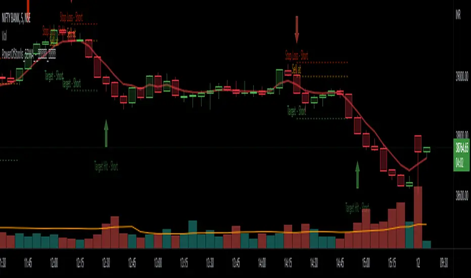
PowerOfStocks_5EMAThis indicator is based of Subhashish Pani's (power of stocks) 5 EMA Strategy.
It plots 5 EMA and Buy/Sell signals with Target & Stoploss levels.
What is Subhashish Pani's (power of stocks) 5 EMA Strategy :-
His strategy is very simple to understand. for intraday use 5 minutes timeframe for selling. You can sell futures, sell call or buy Puts in selling strategy.
What this strategy tries to do is , it tries to catch the tops, so when you sell at top & it turns out to be a reversal point then you can get good profit.
this will hit stop losses often, but stop losses are small and minimum target should be 1:3. but if you stay with the trend you can get big profits.
According to Subhashish Pani this strategy has 60% success rate.
Strategy for Selling (Short future/Call/stock or buy Put)
When ever a Candle closes completely above 5 ema (no part of candle should be touching the 5ema), then that candle should be considered as Alert Candle.
If the next candle is also completely above 5 ema and it has not broken the low of previous alert candle, Then the previous Alert Candle should be ignored and the new candle should be considered as new Alert Candle.
so if this goes on then continue shifting the Alert Candle, but whenever the next candle breaks the low of the Alert Candle we should take the Short trade (Short future/Call/stock or buy Put).
Stoploss will be above high of the Alert Candle and minimum target will be 1:3.
Strategy for Buying (Buy future/Call/stock or sell Put)
When ever a Candle closes completely below 5 ema (no part of candle should be touching the 5ema), then that candle should be considered as Alert Candle.
If the next candle is also completely below 5 ema and it has not broken the high of previous alert candle, Then the previous Alert Candle should be ignored and the new candle should be considered as new Alert Candle.
so if this goes on then continue shifting the Alert Candle, but whenever the next candle breaks the high of the Alert Candle we should take the Long trade (Buy future/Call/stock or sell Put).
Stoploss will be below low of the Alert Candle and minimum target will be 1:3.
Buy/Sell with extra conditions :
it just adds 1 more condition to buying/selling
1. checks if closing of current candle is lower than alert candles closing for Selling & checks if closing of current candle is higher than alert candles closing for Buyling.
This can sometimes save you from false moves but by using this, you can also miss out on big moves as you'll enter trade after candle closing instead of entering at break of high/low.
Note :- According to Subhashish Pani Timeframe for intraday buying should be 15 minutes Timeframe.
If you haven't understood the strategy by reading above description, then search for "Subhashish Pani's (power of stocks) 5 EMA Strategy" on youtube to get a deeper understanding.
Note:- This is not only for Intraday trading , you can use this strategy for Positional/Swing trading as well. If you use this on Monthly Timeframe then it can be very good for Long Term Investing as well.
Rules will be same for all types of trades & Timeframes.
Strategy PnL LibraryLibrary "Strategy_PnL_Library"
TODO: This is a library that helps you learn current pnl of open position and use it to create your own dynamic take profit or stop loss rules based on current level of your profit. It should only be used with strategies.
inTrade()
inTrade: Checks if a position is currently open.
Returns: bool: true for yes, false for no.
notInTrade()
inTrade: Checks if a position is currently open. Interchangeable with inTrade but just here for simple semantics.
Returns: bool: true for yes, false for no.
pnl()
pnl: Calculates current profit or loss of position after the commission. If the strategy is not in trade it will always return na.
Returns: float: Current Profit or Loss of position, positive values for profit, negative values for loss.
entryBars()
entryBars: Checks how many bars it's been since the entry of the position.
Returns: int: Returns a int of strategy entry bars back. Minimum value is always corrected to 1 to avoid lookback errors.
pnlvelocity()
pnlvelocity: Calculates the velocity of pnl by following the change in open profit compared to previous bar. If the strategy is not in trade it will always return na.
Returns: float: Returns a float value of pnl velocity.
pnlacc()
pnlacc: Calculates the acceleration of pnl by following the change in profit velocity compared to previous bar. If the strategy is not in trade it will always return na.
Returns: float: Returns a float value of pnl acceleration.
pnljerk()
pnljerk: Calculates the jerk of pnl by following the change in profit acceleration compared to previous bar. If the strategy is not in trade it will always return na.
Returns: float: Returns a float value of pnl jerk.
pnlhigh()
pnlhigh: Calculates the highest value the pnl has reached since the start of the current position. If the strategy is not in trade it will always return na.
Returns: float: Returns a float highest value the pnl has reached.
pnllow()
pnllow: Calculates the lowest value the pnl has reached since the start of the current position. If the strategy is not in trade it will always return na.
Returns: float: Returns a float lowest value the pnl has reached.
pnldev()
pnldev: Calculates the deviance of the pnl since the start of the current position. If the strategy is not in trade it will always return na.
Returns: float: Returns a float deviance value of the pnl.
pnlvar()
pnlvar: Calculates the variance value of the pnl since the start of the current position. If the strategy is not in trade it will always return na.
Returns: float: Returns a float variance value of the pnl.
pnlstdev()
pnlstdev: Calculates the stdev value of the pnl since the start of the current position. If the strategy is not in trade it will always return na.
Returns: float: Returns a float stdev value of the pnl.
pnlmedian()
pnlmedian: Calculates the median value of the pnl since the start of the current position. If the strategy is not in trade it will always return na.
Returns: float: Returns a float median value of the pnl.
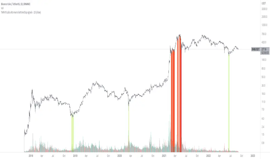
TARVIS Labs - Alts Macro Bottom/Top SignalsSCRIPT DESCRIPTION
PLEASE READ THROUGH THIS CAREFULLY.
This is a script specifically written to help provide indicators from a macro view for ALTS. This script needs to be run on the 1 day. It helps indicate when to accumulate alts, and when its in a bull run when this a bull run top beginning to form with warnings, and a indicator that a top is in. This is described further below.
NOTE - in order to accomodate most alts the script had to be broad enough in its indicators to cover many different scenarios. If you are trading a smaller altcoin I suggest taking a more conservative approach to accumulation.
FAQs:
1. Why is there no accumulation zone showing up before an uptrend?
This could be because the trend has been so strong for this coin that there hasn't been a strong enough signal to accumulate or this could be that the chart doesnt have enough historical data (needs over 2 years) for the indicators to flash green.
2. Why is there no tops shown for a chart Im looking at?
This is either because there isn't enough historical data (needs over 2 years) for the indicators to build or because the altcoin didnt perform as well as the rest of the market. The altcoin has to perform as well as the market over the length of the bull run in order for the signals to show. Typically an altcoin that shows sharp increases and sharp drops shortly after will not have signals show up.
3. The "Potential End of Bull Run Top Indicator" showed up but we weren't near the top yet, why is that?
The alts indicator has to work across many altcoins, and their trends are not all the same. This can lead to the indicator showing but not necessarily being the exact top. The data from the alts macro bottom/top signals should be paired with the "TARVIS Labs bitcoin macro bottom/top signals" indicator for BTC. The reasoning is because if the top is not showing that its in for Bitcoin its likely that the altcoin's top is also not in. You should use the two in tandem to know if the bull run top is very likely in.
ACCUMULATION ZONE INDICATOR - LIGHT GREEN
Description
When we look at the general crypto landscape, the 200d & 300d EMAs are extremely useful. We can use their cross and momentum in order to determine a bottom forming. If the price has fallen over 40% below the 200 day EMA and the 200 day EMA has crossed below the 300d EMA, its a downtrend with a steep fall, which could indicate a good time to accumulate. When we see the 200 day EMA's slope drop drastically (over 5% w/w) it is also a good signal to accumulate.
Strategy for Usage
For alts, the strategy can vary drastically. You need to take into account:
1. the market cap of the altcoin, is it a smaller market cap altcoin or a larger one?
2. historical trend, does it typically trend strongly with a smaller accumulation zone?
Once you've taken these into account you can form a strategy. For example, if the altcoin has had smaller accumulation zones historically you'll want to take advantage of the accumulation zones when they pop up and be more aggressive (say a 30 day accumulation). If the altcoin has historically had longer accumulation zones then you'll want to be more conservative with your strategy and potentially have a 100 day (or even longer) accumulation period. If the altcoin is a smaller market cap alt, you will want to also take that into account. You'll want to likely be more conservative,
STRONG BUY IN ACCUMULATION ZONE INDICATOR - DARK GREEN
Description
We can add to the bottoming signal by looking for strong downtrends inside the bottoming signal. We do this by seeing when the 36 day EMA has a slope decreasing by 2% day/day.
Strategy for Usage
These strong downtrend days can be used to add more to our accumulation strategy. We can add more on these days (ex. double what you were planning to on a typical accumulation day).
LOCAL TOP NEAR BULL RUN TOP INDICATOR - RED
Description
When the 100 week EMA is in a strong uptrend (4% increase w/w) we can look for significant loss of momentum in order to determine if a local top is in near a bull run top. This strategy uses a MACD with 9/36/9 config for the daily chart. We look for the signals momentum loss, when the slope becomes negative.
Strategy for Usage
Ideally the right strategy to use here is to exit the market when this indicator starts. When the indicator ends if the "Potential End of Bull Run Top Indicator" is not showing on the chart you can buy back into the market.
POTENTIAL END OF BULL RUN TOP INDICATOR - DARK RED
Description
When the 100 week EMA is in a strong uptrend (3% increase w/w), and a MACD config of 108/234/9 has a negative signal slope signifying a very large momentum loss, but the 1d 18 EMA is still above the 1d 63 EMA we show this signal.
Strategy for Usage
This is a strong indicator that the top is in, and it potentially being the bull run top. Because alts can vary strongly in their charts, this should be a strong warning but not necessarily a certainty that the bull run is over.
Monthly Returns of a Strategy in a ChartIt's a simple example of how you can present your strategy's monthly performance in a chart.
You maybe know that there is no support of these kind of charts in TradingView so this chart is actually a table object under the hood.
Table visual appearance is customizable, you can change:
Location
Bar Width / High
Colors
Thanks to @MUQWISHI for hard work, for helping me coding it.
It's not about the strategy itself but the way you display returns on your chart. So pls don't critique my choice of the strategy and its performance 🙂
Disclaimer
Please remember that past performance may not be indicative of future results.
Due to various factors, including changing market conditions, the strategy may no longer perform as well as in historical backtesting.
This post and the script don’t provide any financial advice.

ALMA/EMA/SRSI Strategy + IndicatorBack with another great high hit rate strategy!!
Disclaimer* This strategy was sampled using source code written by @ClassicScott , as referred to in the script, there is a clear line where the source code was scripted by myself.
This Strategy consists of three key factors, the ALMA, EMA crossover, and a Stochastic Rsi
ALMA: The Alma is the step line shown, turning green and red at select times. This average value gives general oversight of the macro movement of price action. and this particular one was coded by Mr.ClassicScott.
EMA crossover: At the input screen you are given an option of the fast and slow ema's. The default is solely for the hit rate and correlation to the Alma of this strategy. The arrows you see depicted on the chart are the crossover events happening.
Stochastic Rsi: The Stochastic Rsi is a stochastic value, using data sampled from the rsi. The use of this indicator in my strategy is to prevent entries when too overbought and oversold, as well as closures and vice versa, to prevent holding bags either way.
Fixed % TP: In the input screen you are given a take profit and stop loss percentage, for good R/R the hit rate will take a notch down, but with no R/R it will be near perfect.
How to use this:
Add it to your chart to get the strategy inputs. (The strategy is really only useful on a 15min TF. However the indicator within it can be used on anything at anytime!)
Watch the yellow and aqua moving averages, these are your ema's and crossover's will trigger signals based on your integer inputs.
Find Correlation between other leading indicators, as well as crossover's down/up and a red/green alma.
DO NOT use the arrows as buy/sell signals. These are simply to show ema's are crossing under or over. Momentum indicator's paired with this can be useful to determine if it could be a buy signal or sell signal.
Cheat Code's Notes:
Almost at 1000 boosts!!! I appreciate the support from everyone and I will keep trying my best to deliver quality strategies for the people.
-Cheat Code
BYBIT:BTCUSDT

Smoothed Heikin Ashi Trend on Chart - TraderHalai BACKTESTSmoothed Heikin Ashi Trend on chart - Backtest
This is a backtest of the Smoothed Heikin Ashi Trend indicator, which computes the reverse candle close price required to flip a Heikin Ashi trend from red to green and vice versa. The original indicator can be found in the scripts section of my profile.
This particular back test uses this indicator with a Trend following paradigm with a percentage-based stop loss.
Note, that backtesting performance is not always indicative of future performance, but it does provide some basis for further development and walk-forward / live testing.
Testing was performed on Bitcoin , as this is a primary target market for me to use this kind of strategy.
Sample Backtesting results as of 10th June 2022:
Backtesting parameters:
Position size: 10% of equity
Long stop: 1% below entry
Short stop: 1% above entry
Repainting: Off
Smoothing: SMA
Period: 10
8 Hour:
Number of Trades: 1046
Gross Return: 249.27 %
CAGR Return: 14.04 %
Max Drawdown: 7.9 %
Win percentage: 28.01 %
Profit Factor (Expectancy): 2.019
Average Loss: 0.33 %
Average Win: 1.69 %
Average Time for Loss: 1 day
Average Time for Win: 5.33 days
1 Day:
Number of Trades: 429
Gross Return: 458.4 %
CAGR Return: 15.76 %
Max Drawdown: 6.37 %
Profit Factor (Expectancy): 2.804
Average Loss: 0.8 %
Average Win: 7.2 %
Average Time for Loss: 3 days
Average Time for Win: 16 days
5 Day:
Number of Trades: 69
Gross Return: 1614.9 %
CAGR Return: 26.7 %
Max Drawdown: 5.7 %
Profit Factor (Expectancy): 10.451
Average Loss: 3.64 %
Average Win: 81.17 %
Average Time for Loss: 15 days
Average Time for Win: 85 days
Analysis:
The strategy is typical amongst trend following strategies with a less regular win rate, but where profits are more significant than losses. Most of the losses are in sideways, low volatility markets. This strategy performs better on higher timeframes, where it shows a positive expectancy of the strategy.
The average win was positively impacted by Bitcoin’s earlier smaller market cap, as the percentage wins earlier were higher.
Overall the strategy shows potential for further development and may be suitable for walk-forward testing and out of sample analysis to be considered for a demo trading account.
Note in an actual trading setup, you may wish to use this with volatility filters, combined with support resistance zones for a better setup.
As always, this post/indicator/strategy is not financial advice, and please do your due diligence before trading this live.
Original indicator links:
On chart version -
Oscillator version -
Update - 27/06/2022
Unfortunately, It appears that the original script had been taken down due to auto-moderation because of concerns with no slippage / commission. I have since adjusted the backtest, and re-uploaded to include the following to address these concerns, and show that I am genuinely trying to give back to the community and not mislead anyone:
1) Include commission of 0.1% - to match Binance's maker fees prior to moving to a fee-less model.
2) Include slippage of 10 ticks (This is a realistic slippage figure from searching online for most crypto exchanges)
3) Adjust account balance to 10,000 - since most of us are not millionaires.
The rest of the backtesting parameters are comparable to previous results:
Backtesting parameters:
Initial capital: 10000 dollars
Position size: 10% of equity
Long stop: 2% below entry
Short stop: 2% above entry
Repainting: Off
Smoothing: SMA
Period: 10
Slippage: 10 ticks
Commission: 0.1%
This script still remains to shows viability / profitablity on higher term timeframes (with slightly higher drawdown), and I have included the backtest report below to document my findings:
8 Hour:
Number of Trades: 1082
Gross Return: 233.02%
CAGR Return: 14.04 %
Max Drawdown: 7.9 %
Win percentage: 25.6%
Profit Factor (Expectancy): 1.627
Average Loss: 0.46 %
Average Win: 2.18 %
Average Time for Loss: 1.33 day
Average Time for Win: 7.33 days
Once again, please do your own research and due dillegence before trading this live. This post is for education and information purposes only, and should not be taken as financial advice.

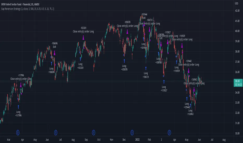
Gap Reversion StrategyToday I am releasing to the community an original short-term, high-probability gap trading strategy, backed by a 20 year backtest. This strategy capitalizes on the mean reverting behavior of equity ETFs, which is largely driven by fear in the market. The strategy buys into that fear at a level that has historically mean reverted within ~5 days. Larry Connors has published useful research and variations of strategies based on this behavior that I would recommend any quantitative trader read.
What it does:
This strategy, for 1 day charts on equity ETFs, looks for an overnight gap down when the RSI is also in/near an oversold position. Then, it places a limit order further below the opening of the gapped-down day. It then exits the position based on a higher RSI level. The limit buy order is cancelled if the price doesn't reach your limit price that day. So, the larger you make the gap and limit %, the less signals you will have.
Features:
Inputs to allow the adjustment of the limit order %, the gap %, and the RSI entry/exit levels.
An option to have the limit order be based on a % of ATR instead of a % of asset price.
An optional filter that can turn-off trades when the VIX is unusually high.
A built in stop.
Built in alerts.
Disclaimer: This is not financial advice. Open-source scripts I publish in the community are largely meant to spark ideas that can be used as building blocks for part of a more robust trade management strategy. If you would like to implement a version of any script, I would recommend making significant additions/modifications to the strategy & risk management functions. If you don’t know how to program in Pine, then hire a Pine-coder. We can help!
Estrategia Larry Connors [JoseMetal]============
ENGLISH
============
- Description:
This strategy is based on the original Larry Connors strategy, using 2 SMAs and RSI.
The strategy has been optimized for better total profit and works better on 4H (tested on BTCUSDT).
LONG:
Price must be ABOVE the slow SMA.
When a candle closes in RSI oversold area, the next candle closes out of the oversold area and the closing price is BELOW the fast SMA = open LONG.
LONG is closed when a candle closes ABOVE the fast SMA.
SHORT:
Price must be BELOW the slow SMA.
When a candle closes in RSI overbought area, the next candle closes out of the overbought area and the closing price is ABOVE the fast SMA = open SHORT.
SHORT is closed when a candle closes BELOW the fast SMA.
*Larry Connor's strategy does NOT use a fixed Stop Loss or Take Profit, as he said, that reduces performance significantly.
- Visual:
Both SMAs (fast and slow) are shown in the chart.
By default, the fast SMA is aqua color, the slow changes between green and red depending on the "trend" (price over slow SMA = bullish, below = bearish).
RSI can't be shown because TradingView doesn't allow to show both overlay and panel indicators, so candles get a RED color when RSI is in OVERBOUGHT area and GREEN when they're on OVERSOLD area to help with that.
Background is colored when conditions are met and a position is going to be open, green for LONGs red for SHORTs.
- Usage and recommendations:
As this is a coded strategy, you don't even have to check for indicators, just open and close trades as the strategy shows.
The original strategy uses a 5 period SMA instead of the 10, and 10/90 for oversold/overbought levels, this has been optimized after the testings and results but feel free to change settings and test by yourself.
Also, the original strategy was developed for daily, but seems to work better en 4H.
- Customization:
As usual I like to make as many aspects of my indicators/strategies customizable, indicators, colors etc., feel free to ask if you feel that something that should be configurable is missing or if you have any ideas to optimize the strategy.
============
ESPAÑOL
============
- Descripción:
Esta estrategia está basada en la estrategia original de Larry Connors, utilizando 2 SMAs y RSI.
La estrategia ha sido optimizada para un mejor beneficio total y funciona mejor en 4H (probado en BTCUSDT).
LONG:
El precio debe estar por encima de la SMA lenta.
Cuando una vela cierra en la zona de sobreventa del RSI, la siguiente vela cierra fuera de la zona de sobreventa y el precio de cierre está POR DEBAJO de la SMA rápida = abre LONG.
Se cierra cuando una vela cierra POR ENCIMA de la SMA rápida.
SHORT:
El precio debe estar POR DEBAJO de la SMA lenta.
Cuando una vela cierra en la zona de sobrecompra del RSI, la siguiente vela cierra fuera de la zona de sobrecompra y el precio de cierre está POR ENCIMA de la SMA rápida = abre SHORT.
Se cierra cuando una vela cierra POR DEBAJO de la SMA rápida.
*La estrategia de Larry Connor NO utiliza un Stop Loss o Take Profit fijo, como él dijo, eso reduce el rendimiento significativamente.
- Visual:
Ambas SMAs (rápida y lenta) se muestran en el gráfico.
Por defecto, la SMA rápida es de color aqua, la lenta cambia entre verde y rojo dependiendo de la "tendencia" (precio por encima de la SMA lenta = alcista, por debajo = bajista).
El RSI no puede mostrarse porque TradingView no permite mostrar tanto los indicadores superpuestos como los del panel, así que las velas obtienen un color ROJO cuando el RSI está en el área de SOBRECOMPRA y VERDE cuando están en el área de VENTA para ayudar a ello.
El fondo se colorea cuando se cumplen las condiciones y se va a abrir una posición, verde para LONGs rojo para SHORTs.
- Uso y recomendaciones:
Como se trata de una estrategia ya programada, ni siquiera hay que comprobar los indicadores, sólo hay que abrir y cerrar las operaciones tal y como muestra la estrategia en el gráfico.
La estrategia original utiliza una SMA de 5 periodos en lugar de 10, y 10/90 para los niveles de sobreventa/sobrecompra, esto ha sido optimizado después de las pruebas y los resultados, pero sé libre de cambiar la configuración y probarla por sí mismo.
Además, la estrategia original fue desarrollada para diario, pero parece funcionar mejor en 4H.
- Personalización:
Como siempre me gusta hacer personalizables todos los aspectos de mis indicadores/estrategias, indicadores, colores, etc., preguntar si notas que falta algo que debería ser configurable o si tienes alguna idea para optimizar la estrategia.

Backtest EngineThis is a simple backtest engine for your trading strategies. The idea behind this script is to make testing new strategies as easy as possible. Parameters such as take profit/stop loss and time period are built into the script and are customisable by the user via the settings interface. The only coding is to set the entry and exit conditions. Users need not touch any code beyond line 30.
For this post, I have used a 50/200 SMA crossover to demonstrate the ease of use for this script.
The features of this script include:
Backtest period start
Number of days until backtest period end
Take profit and stop loss % (via settings)
Programmable long and short entry/exit
Anti duplicate system (for entry conditions that are continuously satisfied, the engine will only make 1 trade until the is exit condition is satisfied).
DISCLAIMER: The strategy in this post is only a placeholder. The TP/SL levels are set to showcase the functionality of the engine and are in no means optimal settings.
Hope this helps! Feel free to ask any questions about the engine and happy coding!

Chandelier Exit - StrategyI created a strategy version for the Chandelier Exit indicator, originally owned by @everget . With the strategy I prepared, you can try both short-long and stop loss - trailing stop and take profit rates. I have also added a date filter feature so that you can test the strategy in the date range you want.
Orjinali @everget 'e ait olan Chandelier Exit indicator için strateji versiyonu oluşturdum. Hazırladığım strateji ile hem short-long deneyebilir hem de zarar durdur - takip eden stop ve kar al oranları denemeleri yapabilirsiniz. İstediğiniz tarih aralığında strateji testi yapabilmeniz için tarih filtre özelliği de ekledim.

RSI StrategyThis RSI strategy will allow you to go long when RSI is overbought and go short when RSI is oversold. You can also change the checked boxes to reverse this. Uncheck "Overbought Go Long & Oversold Go Short" and check "Overbought Go Short & Oversold Go Long" to use this reversed option.
You can also choose to use an ema filter as an additional qualifier for entry. Uncheck "No EMA Filter" and check "Use EMA Filter" if you want to use it.
Be sure to enter slippage and commission into the properties to give you realistic results.
I've also built in backtesting date ranges and the ability to trade only within certain times of day and have it close all trades at the end of that time frame. This is especially useful for day trading stocks. To specify a time from use the format 0930-1100 or whatever your trading hours will be. Check off "Enable Close Trade At End Of Time Frame" to close the trade at the end of your trading hours.
You can also specify a % based take profit and stop loss. Also keep in mind that the way this code is designed if you use the stop loss and/or take profit and it reaches either target and closes, then it will immediately re-enter if the condition for long or short entry is true.
Finally there's custom alert fields so you can send custom alert messages for strategy entry and exit for use with automated trading services. Simply enter your messages in the fields within the strategy properties and then put {{strategy.order.alert_message}} in your alert message body and it will dynamically pull in the appropriate message.

CCI StrategyThis CCI strategy will allow you to enter a long or short off a CCI zero line cross or control entries and exits from custom upper and lower band lengths. You can set a custom upper band which it will buy when it crosses up and then a custom upper band exit which it will sell when it crosses down. For a short you can set a custom lower band which it will short when it crosses down and the custom lower band exit which it will exit the short when it crosses up. Be sure to enter slippage and commission into the properties to give you realistic results.
I've also built in backtesting date ranges and the ability to trade only within certain times of day and have it close all trades at the end of that time frame. This is especially useful for day trading stocks. If you check off "Enter First Trade ASAP" then when using the time frame option it will enter the current trade. If however you uncheck that box and instead check off "Wait To Enter First Trade" it will wait for the trend to change and then enter.
You can also specify a % based take profit and stop loss. Also keep in mind that if you have "Enter First Trade ASAP" checked off and use the stop loss and/or take profit then it will re-enter the current trend again.
Finally there's custom alert fields so you can send custom alert messages for strategy entry and exit for use with automated trading services. Simply enter your messages in the fields within the strategy properties and then put {{strategy.order.alert_message}} in your alert message body and it will dynamically pull in the appropriate message.

Supertrend StrategyThis Supertrend strategy will allow you to enter a long or short from a supertrend trend change. Both ATR period and ATR multiplier are adjustable. If you check off "Change ATR Calculation Method" it will base the calculation off the sma and give you slightly different results, which may work better depending on the asset. Be sure to enter slippage and commission into the properties to give you realistic results.
I've also built in backtesting date ranges and the ability to trade only within certain times of day and have it close all trades at the end of that time frame. This is especially useful for day trading stocks. If you check off "Enter First Trade ASAP" then when using the time frame option it will enter the current trade. If however you uncheck that box and instead check off "Wait To Enter First Trade" it will wait for the trend to change and then enter.
You can also specify a % based take profit and stop loss. In most cases the stop loss is not needed because of the atr based stop that supertrend provides so you could check only take profit and see if it works best to take profit or to let supertrend trend change get you out. Also keep in mind that if you have "Enter First Trade ASAP" checked off and use the stop loss and/or take profit then it will re-enter the current trend again.
Finally there's custom alert fields so you can send custom alert messages for strategy entry and exit for use with automated trading services. Simply enter your messages in the fields within the strategy properties and then put {{strategy.order.alert_message}} in your alert message body and it will dynamically pull in the appropriate message.

Multi MA Trend Following Strategy TemplateTrend following is one of the better known technical trading strategies. But, which trend should you follow? Today I am sharing with the community a trend following template script that includes a selection of over 20 different trends / regressions. Some of these are in the Pine library, and some have been custom coded and contributed over time by the beloved Pine Coder community.
How it works:
This template will plot any of the 20+ trends that you can select in the settings. The strategy component will buy if the trend line is moving up, and will sell if it moves down. If the line is green that indicates that the trend is higher than the prior bar. If the line is red that indicates that the trend is lower than the prior bar. This script is different from many moving average scripts in that it follows the trend itself and doesn't look for a cross of multiple trends.
How to use it:
When wanting to trend follow an instrument, you can use this template to help identify what approach you might want to take and/or which indicator you might want to use. You can also modify the strategy as you see fit and make use of the 20+ incorporated indicators. Incorporate your trade and risk management strategy, or use it as an indicator.
Disclaimer: Open source scripts I publish in the community are largely meant to spark ideas that can be used as building blocks for part of a more robust trade management strategy. Even though this example script might beat buy and hold over the back-test time-frame, I wouldn't advise using it as a stand-alone strategy without significant additions/modifications to the strategy and risk management functions.

Combo Backtest 123 Reversal & TEMA1This is combo strategies for get a cumulative signal.
First strategy
This System was created from the Book "How I Tripled My Money In The
Futures Market" by Ulf Jensen, Page 183. This is reverse type of strategies.
The strategy buys at market, if close price is higher than the previous close
during 2 days and the meaning of 9-days Stochastic Slow Oscillator is lower than 50.
The strategy sells at market, if close price is lower than the previous close price
during 2 days and the meaning of 9-days Stochastic Fast Oscillator is higher than 50.
Second strategy
This study plots the TEMA1 indicator. TEMA1 ia s triple MA (Moving Average),
and is calculated as 3*MA - (3*MA(MA)) + (MA(MA(MA)))
WARNING:
- For purpose educate only
- This script to change bars colors.
TradingGroundhog - Strategy & Fractal V1#-- Public Strategy - No Repaint - Fractals -- Short term
Here I come with another script, more simple than Wavetrend V1. You will love it.
#-- Synopsis --
Another simple idea, on a small time frame (15 min) we buy when the opening price goes below a Bottom fractals and sell when it goes over a Top fractals, but as this script do not use Wavetrends. You should stop by your self to use the script during long lasting downtrends.
I developed the strategy using BTC /EUR 3 MIN BINANCE but it can be applied to many other cryptos, I don't know for forex or others. You can use it for short term (to a month of uptrend) and automated trading.
#-- Graph reading --
And now, how to read it ?
Fractals:
Yellow Flags occur when the opening price goes below a Bottom fractal , it means Buy.
White Flags appear when the opening price goes over a Top fractal , it means Sell.
#-- Parameters --
*** Parameters have been intensively optimized using 10 cryptocurrency markets in order to have potent efficiency for each of them. I would recommend to only change the Can Be touch parameter. For the others, I don't recommend any modifications. The idea behind the script is to be able to switch between markets without having to optimize parameters, less work, easy to target active crypto and therefor limit the risks. ***
Can be touch :
'Filter fractals' : Activate or Disable the filtering fractal operation. If Enable, buy during less risky periods. (Activate is often better)
Can be touch but not necessary :
'VolumeMA' : The Volume corrector used by the fractals
'Extreme window' : The number of price individuals to look for if we want to remove extreme fractals.
Not to touch :
'Long Sop Loss (%)' : The minimal difference of price between a Fractal bottom and the opening price to buy.
#-- Time frame --
Should be used with the following time frames depending on the necessity:
1 MIN
3 MIN (Preferred with the parameters set)
5 MIN
#-- Last words --
The script can be set up to send Tradingview signals to 3comma just by adding comment = " " in strategy.close_all() and strategy.entry().
Good trades !
Disclaimer (As it should always be one to any script)
***
This script is intended for and only to be used for personal purposes only. No such information provided by it constitutes advice or a recommendation for any investment or trading strategy for any specific person. There is no guarantee presented or implied as to the accuracy of specific forecasts, projections, or predictive statements offered by the script. Users of the script agree that its original developer does not take responsibility for any of your investment decisions. Please seek professional advice before trading.
***
# Here are the results from the 20rst of September 2021 with 100% of equity on the BTC /EUR 3 Min and with a capital of 10 000 EUR. So almost, one month.
# As I saw, it goes from +30% to more than +160% (the great SHIB) depending on the selected crypto. It may be negative if you spot a downtrend.
